Source Analysis Across Screening Phases
2026-02-17
Source:vignettes/citesource_working_example.rmd
citesource_working_example.rmdAbout this vignette
In order to complete a reliable systematic search one must include multiple resources to ensure the inclusion of all relevant studies. The exact number of sources that are necessary for a thorough search can vary depending on the topic, type of review, etc. Along with the selection and search of traditional literature sources, other methods such as hand searching relevant journals, citation chasing/snowballing, searching websites, etc. can be used to minimize the risk of missing relevant studies. But how important is that extra database? How much return are you getting from the weeks worth of combing through websites? Did that open resource perform just perform as well as (or better than) the one your library/institution pays 500k/year for? How much time could you save if you had these answers? Wouldn’t knowing the answers to these questions give us a better understanding of HOW to conduct our searches? Wouldn’t it be great it we could speed up the process without impacting its quality, better yet, improve our understanding while making the process faster?
These were some of the main questions that our team wanted to answer. The goal of this vignette (which we’d love your feedback on) is to show you how CiteSource can help you gather information on the ways sources and methods impact a review. The data in this vignette is based on a subset of data from an actual project. In it, we’ll walk through how CiteSource can import original search results, compare those information sources and methods, and determine how they contributed to the final review.
If you have any questions, feedback, ideas, etc. about this vignette or others be sure to check out our discussion board on github!
1. Installation of packages and loading libraries
Use the following code to install CiteSource. Currently, CiteSource lives on GitHub, so you may need to first install the remotes package. This vignette also uses functions from the ggplot2 and dplyr packages.
#Install the remotes packages to enable installation from GitHub
#install.packages("remotes")
#library(remotes)

#Install CiteSource
#remotes::install_github("ESHackathon/CiteSource")

#Load the necessary libraries
library(CiteSource)
library(dplyr)
2. Import Reference Files and Add Custom Metadata
Users can import multiple .ris or .bib files into CiteSource, which they can then label with three custom metadata fields: cite_source, cite_string, and cite_label.
Using the cite_source field, the user can label individual files with source information such as database or platform. Beyond source information, users may also use the cite_source field to provide search results using various search methodologies.
The second field, cite_label, can be used to apply yet another variable. This label was intended to be used in combination with the label cite_source, to track the inclusion or exclusion of citations from a specific source over the course of title/abstract and full text screening.
As a note, CiteSource does provide a third metadata field, cite_string, which can be used to specify another attribute or variable. For example, a use of cite_source and cite_string may be to examine the unique and crossover citations that occur between databases, while simultaneously evaluating unique search string results. While it’s possible to use cite_string, we have not fully integrated this third field into any of our tables and plots and it is not used in this vignette. As we continue to develop CiteSource and get feedback from users, we’ll continue to update this and other vignettes.
Indicate file location
#Import citation files from a folder
citation_files <- list.files(path = file.path("../vignettes/working_example_data"), pattern = "\\.ris", full.names = TRUE)

#Print citation_files to double check the order in which R imported the files.
citation_files
#>  [1] "../vignettes/working_example_data/AGRIS.ris"
#>  [2] "../vignettes/working_example_data/CAB.ris"
#>  [3] "../vignettes/working_example_data/EconLit.ris"
#>  [4] "../vignettes/working_example_data/Final.ris"
#>  [5] "../vignettes/working_example_data/GreenFile.ris"
#>  [6] "../vignettes/working_example_data/McK.ris"
#>  [7] "../vignettes/working_example_data/RM.ris"
#>  [8] "../vignettes/working_example_data/TiAb.ris"
#>  [9] "../vignettes/working_example_data/WoS_early.ris"
#> [10] "../vignettes/working_example_data/WoS_later.ris"
3. Read in citation files and add custom metadata
Prior to importing files into CiteSource, it is recommended that users import raw .ris/.bib files into a citation management software such as EndNote or Zotero and combine multiple citation files from each individual source. This can reduce complication and assist with applying metadata. Features such as EndNote’s “find reference updates” can also ensure that citations are more complete by filling in missing metadata fields.
In this example, we read in the citaiton files and tag the citation files with the resource they came from using the cite_source field. The two citation files labeled NA represent the file from included papers after title/abstract screening and the file of the included papers after full-text screening and therefore are not assigned a source. The cite_label tag is being used to tag files with “search” (the initial search results), “screened” (included papers after TI/AB screening), and “final” (papers included after full-text screening).
# Import citation files from folder
citation_files <- list.files(path = "working_example_data", pattern = "\\.ris", full.names = TRUE)

# Print list of citation files to console
citation_files
#>  [1] "working_example_data/AGRIS.ris"     "working_example_data/CAB.ris"
#>  [3] "working_example_data/EconLit.ris"   "working_example_data/Final.ris"
#>  [5] "working_example_data/GreenFile.ris" "working_example_data/McK.ris"
#>  [7] "working_example_data/RM.ris"        "working_example_data/TiAb.ris"
#>  [9] "working_example_data/WoS_early.ris" "working_example_data/WoS_later.ris"

# Set the path to the directory containing the citation files
file_path <- "../vignettes/working_example_data/"

metadata_tbl <- tibble::tribble(
  ~files,           ~cite_sources, ~cite_labels,
   "AGRIS.ris",      "AGRIS",       "search",
   "CAB.ris",        "CAB",         "search",
   "EconLit.ris",    "EconLit",     "search",
   "Final.ris",       NA,           "final",
   "GreenFile.ris",  "GreenFile",   "search",
   "McK.ris",        "Method1",     "search",
   "RM.ris",         "Method2",     "search",
   "TiAb.ris",        NA,           "screened",
   "WoS_early.ris",  "WoS",         "search",
   "WoS_later.ris",  "WoS",         "search"
) %>%

dplyr::mutate(files = paste0(file_path, files))
citations <- read_citations(metadata = metadata_tbl)
#> Importing files ■■■                                6%
#> Importing files ■■■                                8%
#> Importing files ■■■■                               9%
#> Import completed - with the following details:
#>             file cite_source cite_string cite_label citations
#> 1      AGRIS.ris       AGRIS        <NA>     search        12
#> 2        CAB.ris         CAB        <NA>     search       687
#> 3    EconLit.ris     EconLit        <NA>     search        50
#> 4      Final.ris        <NA>        <NA>      final       242
#> 5  GreenFile.ris   GreenFile        <NA>     search       139
#> 6        McK.ris     Method1        <NA>     search      2656
#> 7         RM.ris     Method2        <NA>     search       530
#> 8       TiAb.ris        <NA>        <NA>   screened      1573
#> 9  WoS_early.ris         WoS        <NA>     search      2550
#> 10 WoS_later.ris         WoS        <NA>     search       736
4. Deduplication & Identifying Crossover Records
CiteSource allows users to merge duplicate records, while maintaining information in the cite_source, cite_label,and cite_string fields.
Note that duplicates are assumed to published in the same source, so pre-prints and similar results will not be identified as duplicates.
unique_citations <- dedup_citations(citations)
#> Registered S3 method overwritten by 'synthesisr':
#>   method                     from
#>   as.data.frame.bibliography CiteSource
#> formatting data...
#> identifying potential duplicates...
#> identified duplicates!
#> flagging potential pairs for manual dedup...
#> Joining with `by = join_by(duplicate_id.x, duplicate_id.y)`
#> 9175 citations loaded...
#> 3323 duplicate citations removed...
#> 5852 unique citations remaining!

# Count number of unique and non-unique citations from different sources and labels
n_unique <- count_unique(unique_citations)

# Create dataframe indicating occurrence of records across sources
source_comparison <- compare_sources(unique_citations, comp_type = "sources")

# initial upload/post internal deduplication table creation
initial_counts<-record_counts(unique_citations, citations, "cite_source")
record_counts_table(initial_counts)| Record Counts | ||
| Records Imported1 | Distinct Records2 | |
|---|---|---|
| AGRIS | 12 | 12 |
| CAB | 687 | 687 |
| EconLit | 50 | 50 |
| GreenFile | 139 | 139 |
| Method1 | 2656 | 2367 |
| Method2 | 530 | 472 |
| WoS | 3286 | 2989 |
| Total | 7360 | 6716 |
| 1 Number of records imported from each source. | ||
| 2 Number of records after internal source deduplication | ||
5. Analyzing Sources & Methods
When teams are selecting databases for inclusion in a review it can be extremely difficult to determine the best resources and determine the ROI in terms of the time it takes to apply searches. This is especially true in fields where research relies on cross-disciplinary resources. By tracking and reporting where/how each citation was found, the evidence synthesis community could in turn track the utility of various databases/platforms and identify the most relevant resources as it relates to their research topic. This idea can be extended to search string comparison as well as various search strategies and methodologies.
Plot overlap as a heatmap matrix
CiteSource performs citation analysis and deduplication within each source file, prior to comparing sources across source files. This heatmap shows the number of citations unique to each source at the top of the source’s column. The heatmap also provides a count of citations that were found at the intersection of each source.
In this case, you can see that the source tag “Method 1” only shows 2364 records, while the initial .ris file contained 2656 citations. This means that CiteSource identified duplicate references within that citation list. The 2364 remaining citations are attributed to this source. Looking at the source Greenfile, we can see that CiteSource did not find any duplicate citations within this source as both counts read 139.
my_heatmap <- plot_source_overlap_heatmap(source_comparison)

my_heatmap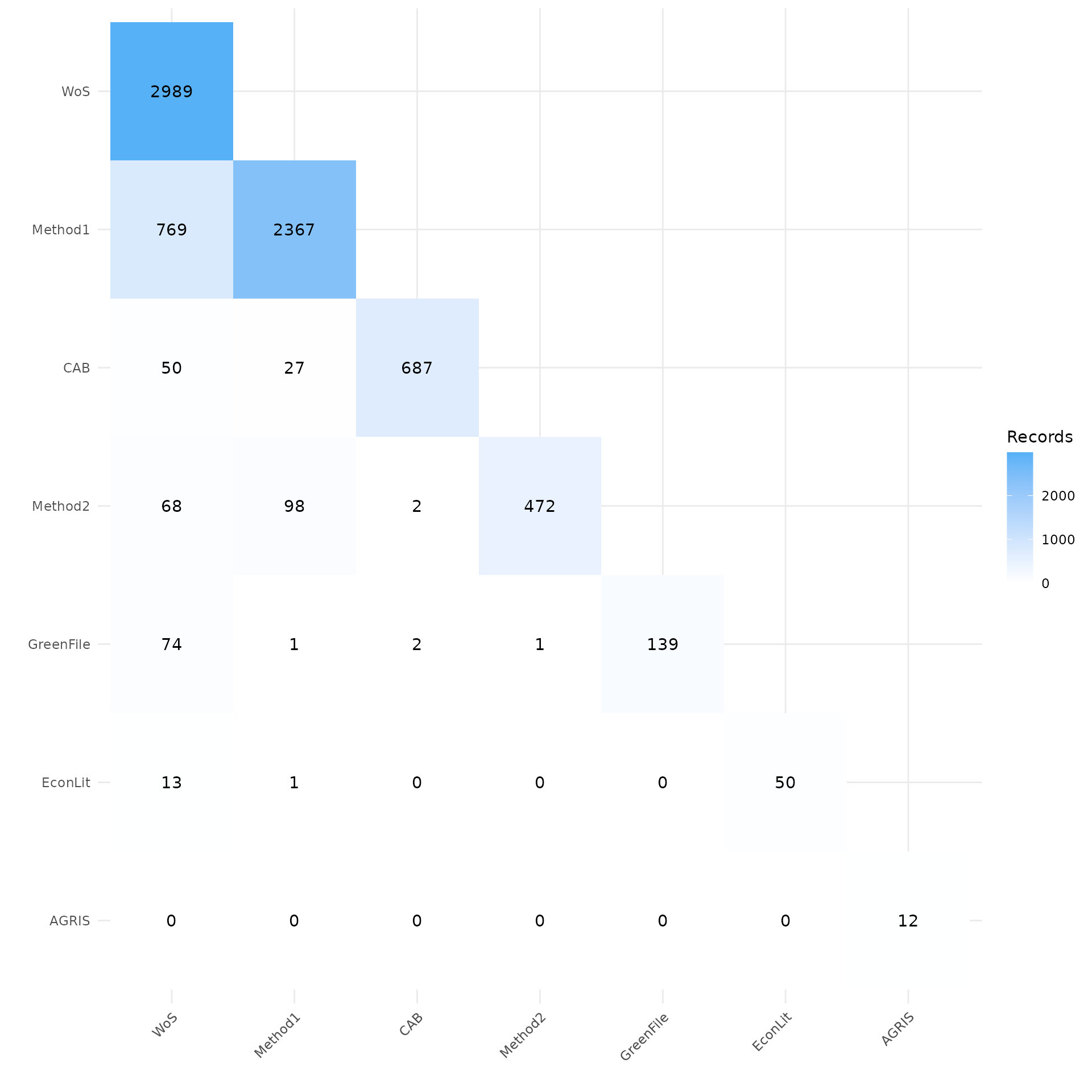
Plot overlap as a heatmap matrix as percentage
The following heatmap provides an overview of the overlapping citations by percent of each source’s count. For example the EconLit source contains 50 citations. Of those 50 we can see on the previous heatmap that 8 of these citations were also in the source WoSE, which represents 16% of the citations from EconLit. On the other hand the same 8 citations only represent .3% of the total citations from WoSE. (currently this chart is set to display only whole numbers - we are considering changing this to display to the first decimal)
my_heatmap_percent <- plot_source_overlap_heatmap(source_comparison, plot_type = "percentages")

my_heatmap_percent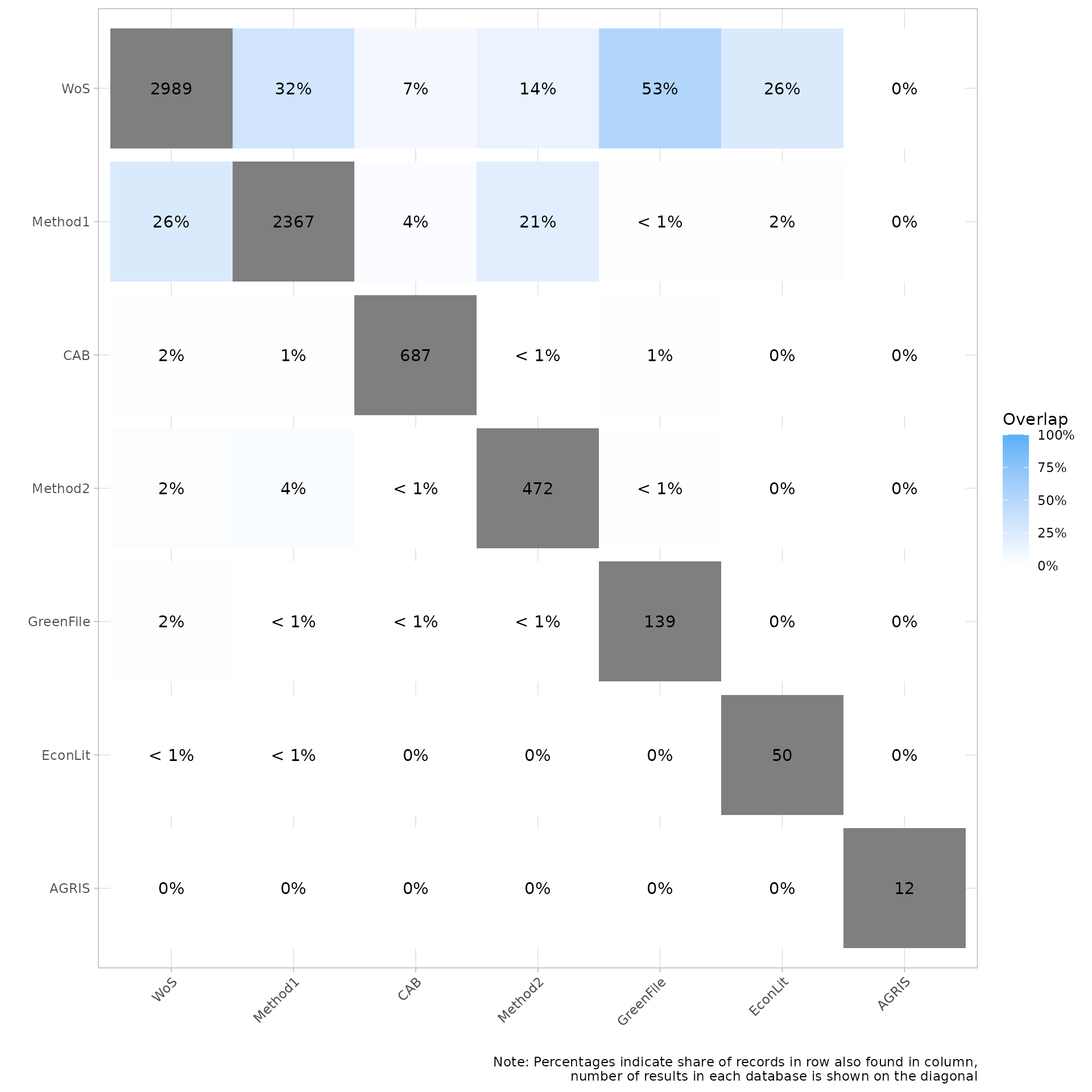
Plot overlap as an upset plot
my_upset_plot <- plot_source_overlap_upset(source_comparison, decreasing = c(TRUE, TRUE))
#> Plotting a large number of groups. Consider reducing nset or sub-setting the data.

my_upset_plot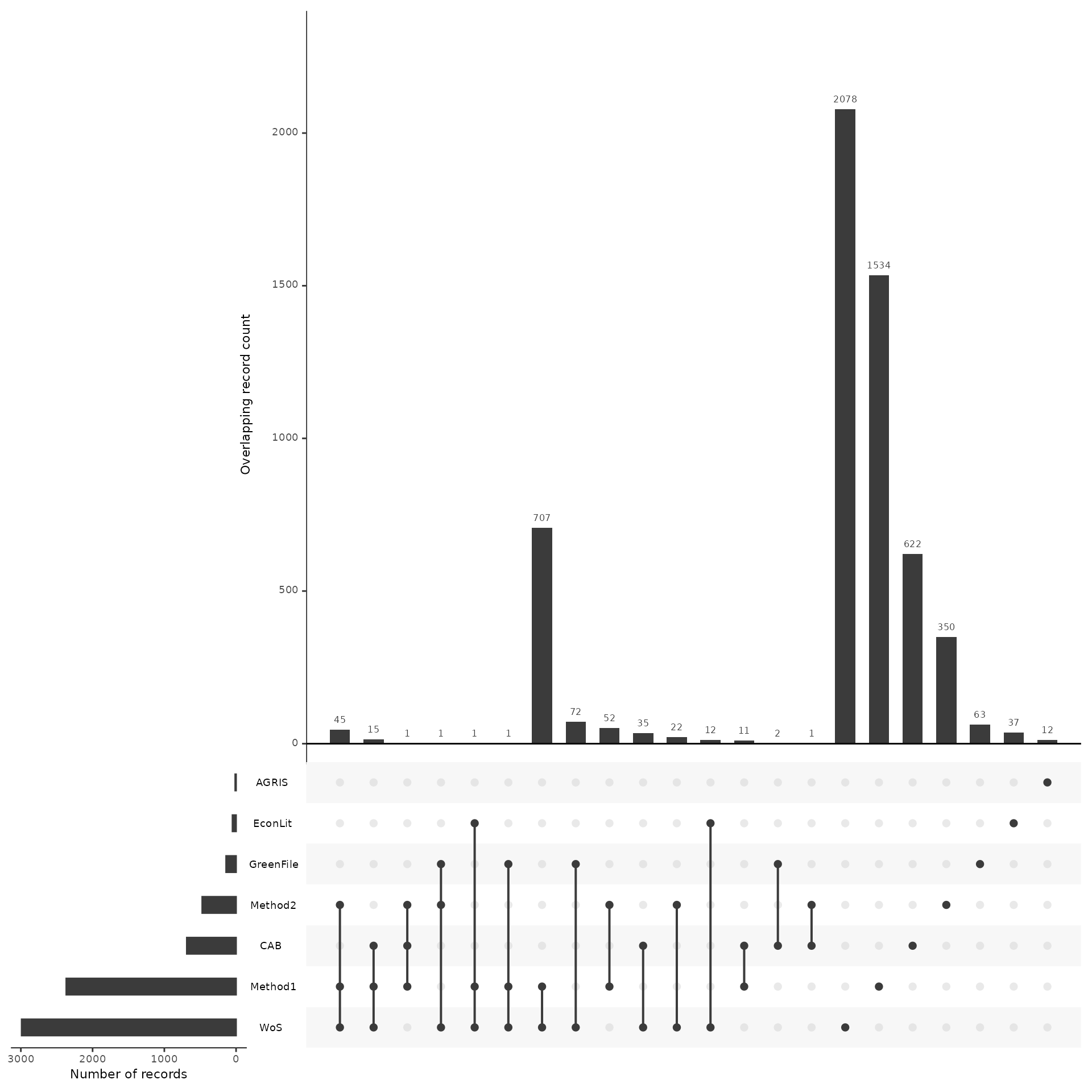
6. Analyzing records after screening
Once the title and abstract screening has been completed or once the final papers have been selected, users can analyze the contributions of each source or search method to these screening phases to better understand their impact on the review. By using the “cite_source” data along with the “cite_label” data, users can analyze the number of overlapping/unique records from each source or method.
Assessing contribution of sources by review stage
my_contributions <- plot_contributions(n_unique,
  center = TRUE,
  bar_order = c("search", "screened", "final")
)

my_contributions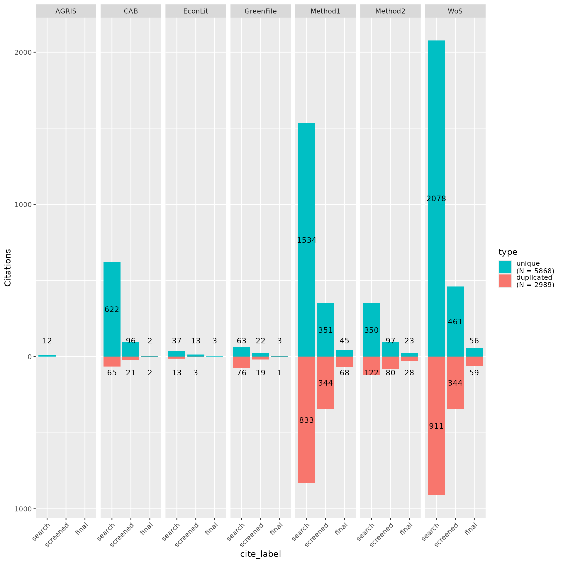
Analyzing Precision/Sensitivity
In addition to the above visualizations, it may be useful to export tables for additional analysis. Presenting data in the form of a search summary table can provide an overview of each source’s impact as well as precision and sensitivity (see Bethel et al. 2021 for more about search summary tables).
calculated_counts<-calculate_record_counts(unique_citations, citations, n_unique, "cite_source")
record_summary_table(calculated_counts)| Record Counts | |||||||
| Records Imported1 | Distinct Records2 | Unique records3 | Non-unique Records4 | Records Contributed %5 | Unique Records Contributed %6 | Unique Records %7 | |
|---|---|---|---|---|---|---|---|
| AGRIS | 12 | 12 | 12 | 0 | 0.2% | 0.3% | 100.0% |
| CAB | 687 | 687 | 622 | 65 | 10.2% | 13.2% | 90.5% |
| EconLit | 50 | 50 | 37 | 13 | 0.7% | 0.8% | 74.0% |
| GreenFile | 139 | 139 | 63 | 76 | 2.1% | 1.3% | 45.3% |
| Method1 | 2656 | 2367 | 1534 | 833 | 35.2% | 32.7% | 64.8% |
| Method2 | 530 | 472 | 350 | 122 | 7.0% | 7.5% | 74.2% |
| WoS | 3286 | 2989 | 2078 | 911 | 44.5% | 44.3% | 69.5% |
| Total | 7360 | 8 5852 | 4696 | 2020 | NA | NA | NA |
| 1 Number of raw records imported from each database. | |||||||
| 2 Number of records after internal source deduplication | |||||||
| 3 Number of records not found in another source. | |||||||
| 4 Number of records found in at least one other source. | |||||||
| 5 Percent distinct records contributed to the total number of distinct records. | |||||||
| 6 Percent of unique records contributed to the total unique records. | |||||||
| 7 Percentage of records that were unique from each source. | |||||||
| 8 Total citations discoverd (after internal and cross-source deduplication) | |||||||
phase_counts<-calculate_phase_count(unique_citations, citations, "cite_source")
precision_sensitivity_table(phase_counts)| Record Counts & Precision/Sensitivity | |||||
| Distinct Records1 | Screened Included2 | Final Included3 | Precision4 | Sensitivity/Recall5 | |
|---|---|---|---|---|---|
| AGRIS | 12 | 0 | 0 | 0 | 0 |
| CAB | 687 | 117 | 4 | 0.58 | 1.65 |
| EconLit | 50 | 16 | 3 | 6 | 1.24 |
| GreenFile | 139 | 41 | 4 | 2.88 | 1.65 |
| Method1 | 2367 | 695 | 113 | 4.77 | 46.69 |
| Method2 | 472 | 177 | 51 | 10.81 | 21.07 |
| WoS | 2989 | 805 | 115 | 3.85 | 47.52 |
| Total | 6 5852 | 7 1573 | 8 242 | 9 4.14 | NA |
| 1 Number of records after internal source deduplication | |||||
| 2 Number of citations included after title/abstract screening | |||||
| 3 Number of citations included after full text screening | |||||
| 4 Number of final included citations / Number of distinct records | |||||
| 5 Number of final included citations / Total number of final included citations | |||||
| 6 Total citations discoverd (after internal and cross-source deduplication) | |||||
| 7 Total citations included after Ti/Ab Screening | |||||
| 8 Total citations included after full text screening | |||||
| 9 Overall Precision = Number of final included citations / Total distinct records | |||||
Creating a Citation Record Table
Another useful table that can be exported as a .csv is the record-level table. This table allows users to quickly identify which individual citations in the screened and/or final records were present/absent from each source. The source tag is the default (include = “sources”), but can be replaced or expanded with ‘labels’ and/or ‘strings’
unique_citations %>%
  dplyr::filter(stringr::str_detect(cite_label, "final")) %>%
  record_level_table(return = "DT")
7. Exporting for further analysis
We may want to export our deduplicated set of results (or any of our
dataframes) for further analysis or to save them in a convenient format
for subsequent use. CiteSource offers a set of export functions called
export_csv, export_ris and
export_bib that will save dataframes as a .csv file, .ris
file or .bib file, respectively.
You can then reimport exported files to pick up a project or analysis without having to start from scratch, or after making manual adjustments (such as adding missing abstract data) to a file.
Generate a .csv file. The separate argument can be used to create separate columns for cite_source, cite_label or cite_string to facilitate analysis.
#export_csv(unique_citations, filename = "citesource_working_example.csv", separate = "cite_source")Generate a .ris file and indicate custom field location for cite_source, cite_label or cite_string. In this example, we’ll be using EndNote, so we put cite_sources in the DB field, which will appear as the Name of Database field in EndNote and cite_labels into C5, which will appear as the Custom 5 metadata field in EndNote.
#export_ris(unique_citations, filename = "citesource_working_example.ris", source_field = "DB", label_field = "C5")Generate a bibtex file and include data from cite_source, cite_label or cite_string.
#export_bib(unique_citations, filename = "citesource_working_example.bib", include = c("sources", "labels", "strings"))In order to reimport a .csv or a .ris you can use the follwowing. Here is an example of how you would reimport the file if it were on your desktop
#citesource_working_example <-reimport_csv("citesource_working_example.csv")

#citesource_working_example <-reimport_ris("citesource_working_example.ris")